
Predicting Healthcare Cost
Among Medicare Beneficiaries in Massachusetts
Among Medicare Beneficiaries in Massachusetts
The rising cost of healthcare is one of the world’s most important problems. Healthcare policy researchers have devoted much effort toward finding solutions to the fast growth in health care spending over the past decade. Research has provided evidence that the growth is linked to modifiable population risk factors such as obesity and stress. Rising disease prevalence and new medical treatments account for nearly two-thirds of the rising spending. As MA residents, we are directly concerned with how the state controls its healthcare cost. As one article in Boston Globe put it, “The soaring costs of insuring the state’s poorest residents drove health care spending in MA up 4.8 percent last year, double the rate of growth in 2013, dealing a setback to the state’s effort to control medical costs.” /
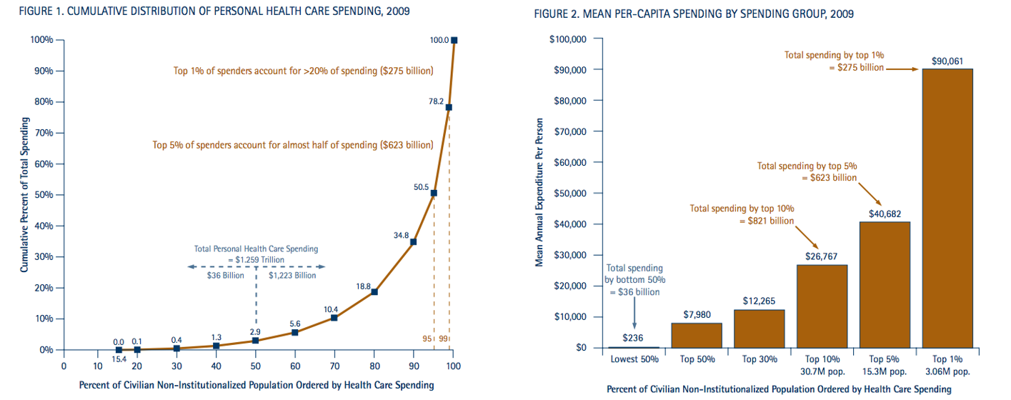 Source: NIHCM Foundation Data Brief 2012. http://www.nihcm.org/
Therefore, predicting such costs with accuracy is a significant first step in addressing this problem, and may reveal insights into the nature of the key drivers of costs.
Our data source comes from Centers for Medicare and Medicaid Limited Data Set Files, which records medicare claims happened in all medical settings. The original data files we will derive our analytic dataset from, includes: Denominator File, Inpatient File, Outpatient Fil, Carrier File, Skilled Nursing Facility File, Hospice File, Home Health Agency File, and Durable Medical Equipment File. They cover all medical claims and associated costs for Medicare FFS beneficiaries.
So let us explain what claims data is. Medical claims are generated when a patient visits a doctor. They include diagnosis codes, procedure codes, as well as costs. Claims data are electronically available, they are standardized and well-established codes. However, since humans generate them, they are 100% accurate. Also, claims for hospital visits can be vague. These limitations push us to work harder to find signals from noise. Or in other words, we want to find valuable information from chaos reality. This is what we do: Reality Mining!
In creating analytic dataset for use, our objective is to model future costs with past medical history. We randomly select 20% sample of Massachusetts Medicare Fee-For-Service Beneficiaries who was fully-insured during 2012 and 2013 and who did not die. We use claims during 01/01/2012 to 12/31/2012 to create chronic disease indicators, diagnosis indicators, and procedures indicators, and we use claims during 01/01/2013 to 12/31/2013 to create binary indicator for top 10% high cost patients.
Our data prepare phase includes collecting claims associated with the same patients and aggregate information to patient-level. Our final analytic dataset includes:
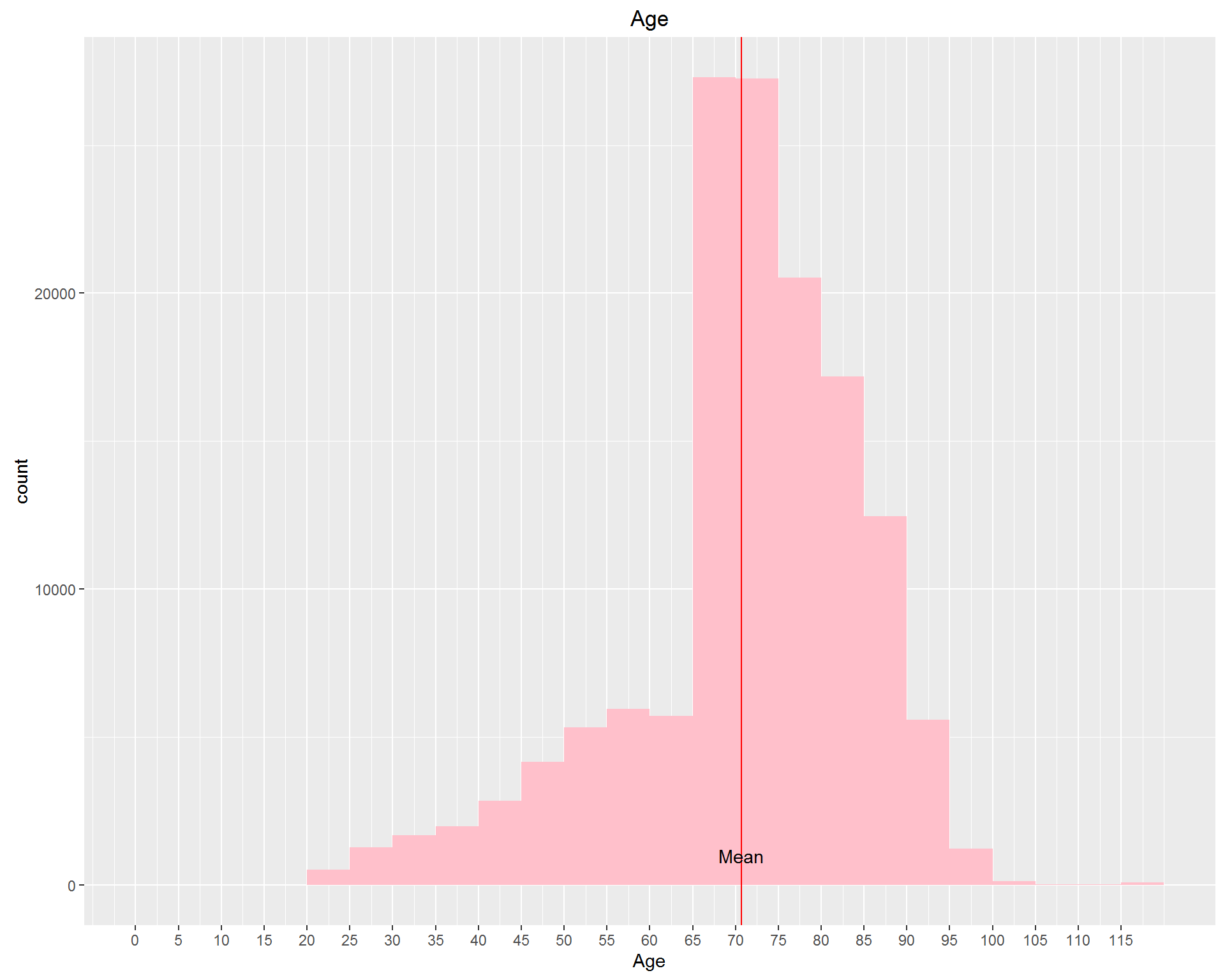
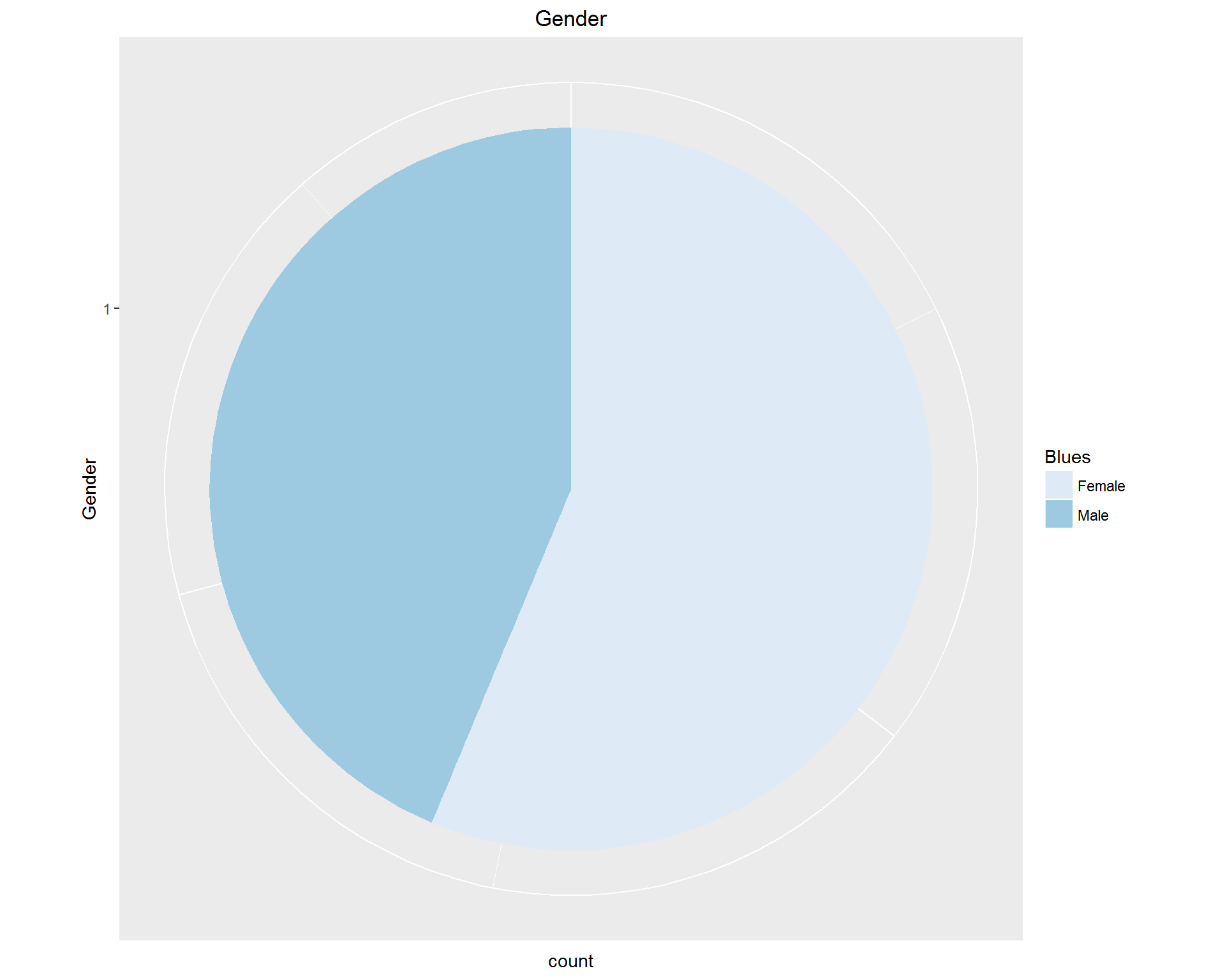
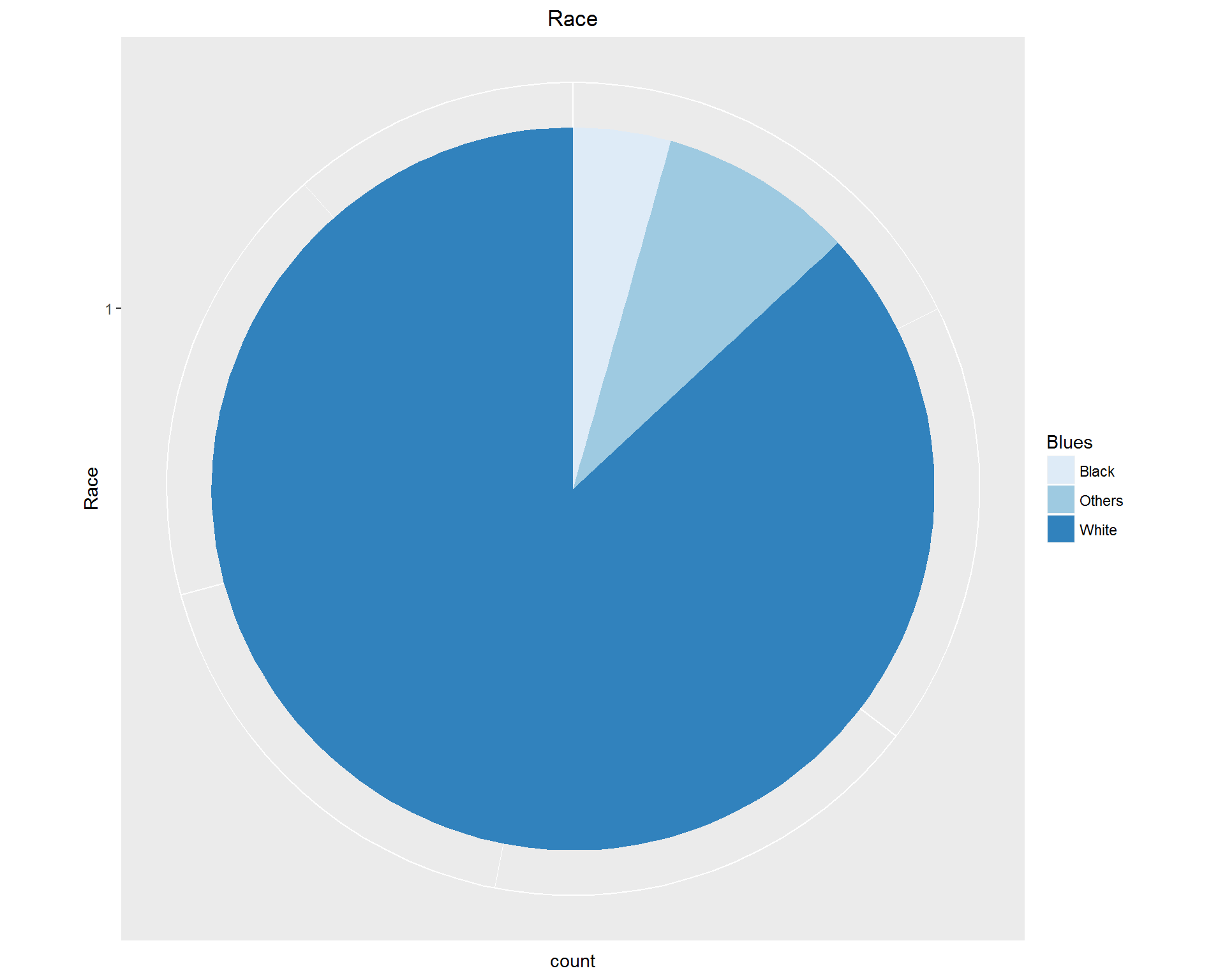
First, we look at demographic information: Age, Gender, and Race. These can be seen in the images above. We're dealing with an older, mostly white population with more women than men represented.
Second, we look at the relationship between patients’ 2012 medical cost and 2013 medical cost. We anticipate the correlation is strong, because older people with weaker health tend to have chronically high need of medical care.
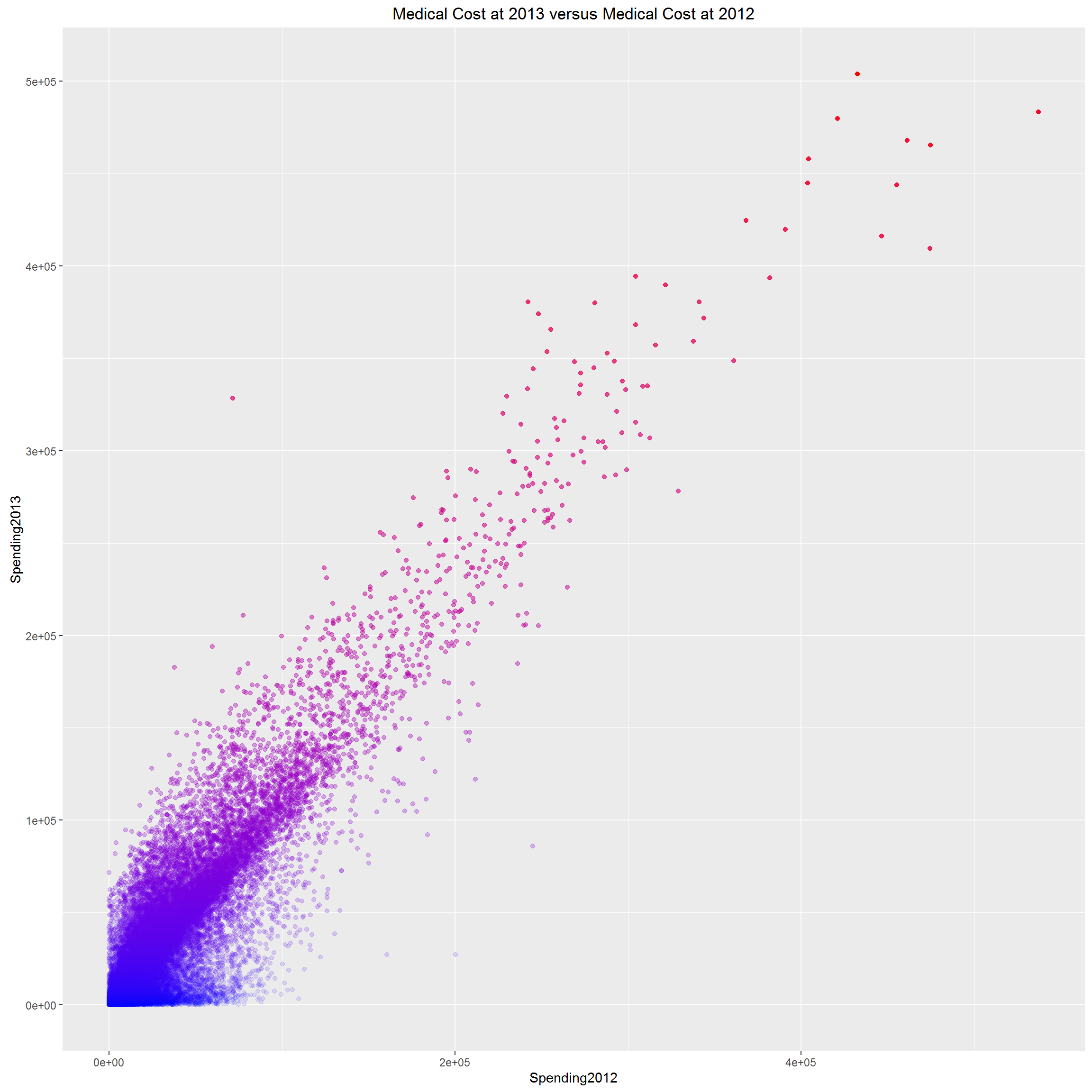
We can clearly see that, spending pattern is so consistent for Medicare beneficiaries, in the sense that, two subsequent years’ medical costs could nearly perfectly predict each other. However, we don’t know if it is true for general population. At least, it tells us that, for Medicare beneficiaries, typically older population >=65, if we know their past year’s medical cost, their next year’s cost is predictable with high confidence. And some people (red dots) are consistently high medical resource utilizers; while others (blue dots) are consistently 0 utilizers, they are healthy population; the rest falling in the middle are relatively healthy and would not drive the total healthcare cost up dramatically. The red dots are the population we care most about. They are the population with more chronic diseases which need long-term medical assistance.
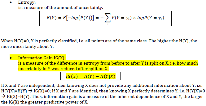
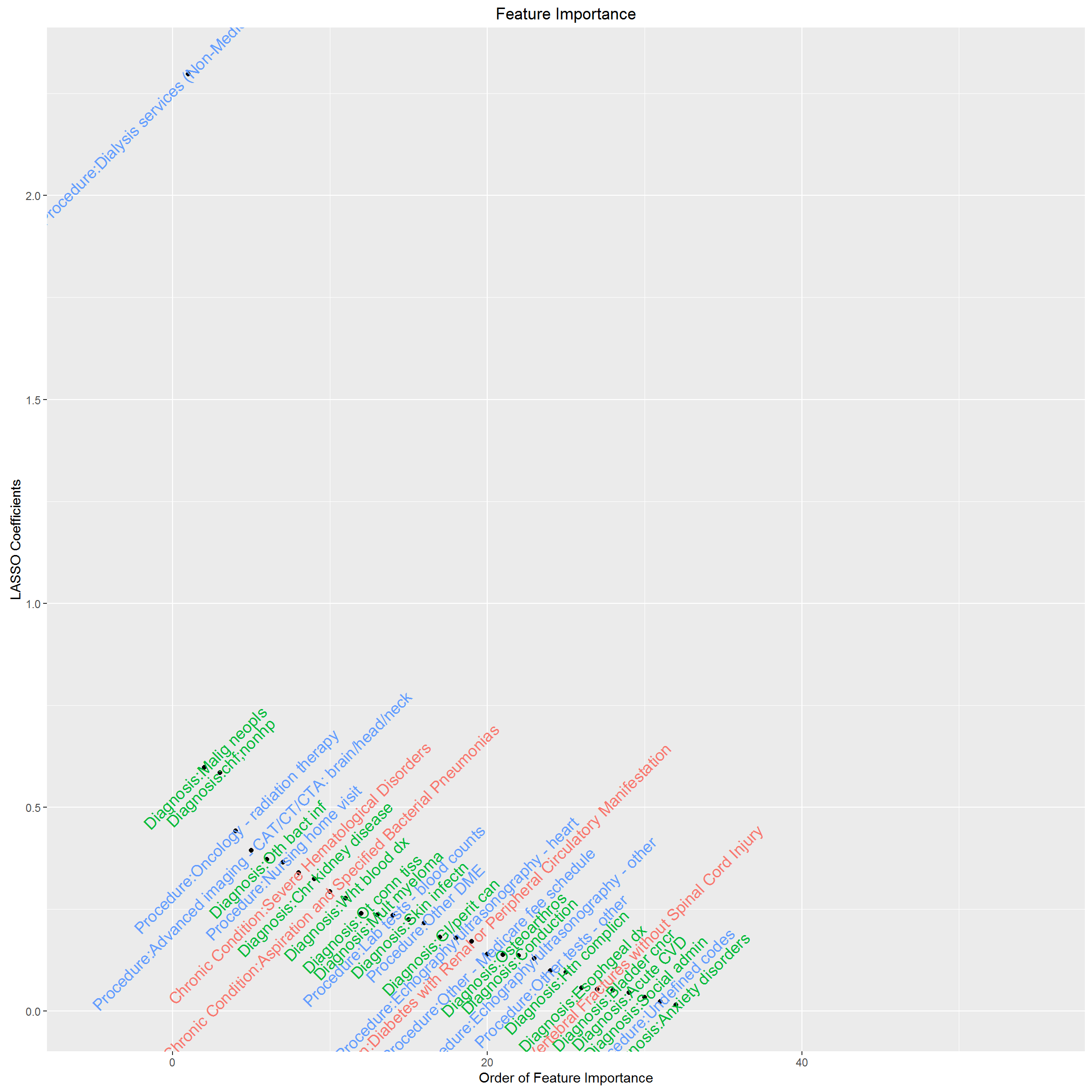
The dataset contains 70 chronic condition indicators (HCC), 283 Diagnosis Groups (DXCCS), 105 Procedure categories, which leads to 458 potential features. Technically, we need to reduce “the curse of dimensionality”; practically, if we build an algorithm that only works if we know all these information about a patient, it would be impossible to implement at clinical setting, and would also provide no insight into who will be high resource utilizers and what their characteristics are. Thus, the first task for us is to select features with high predictive power, and reduce the “curse of dimensionality”. The usual statistics Pearson’s correlation coefficient is a measure of linear relationship for continuous variables, thus inappropriate for our case. We’ll use “information gain” or “Entropy” as a measure of predictive power for individual feature.
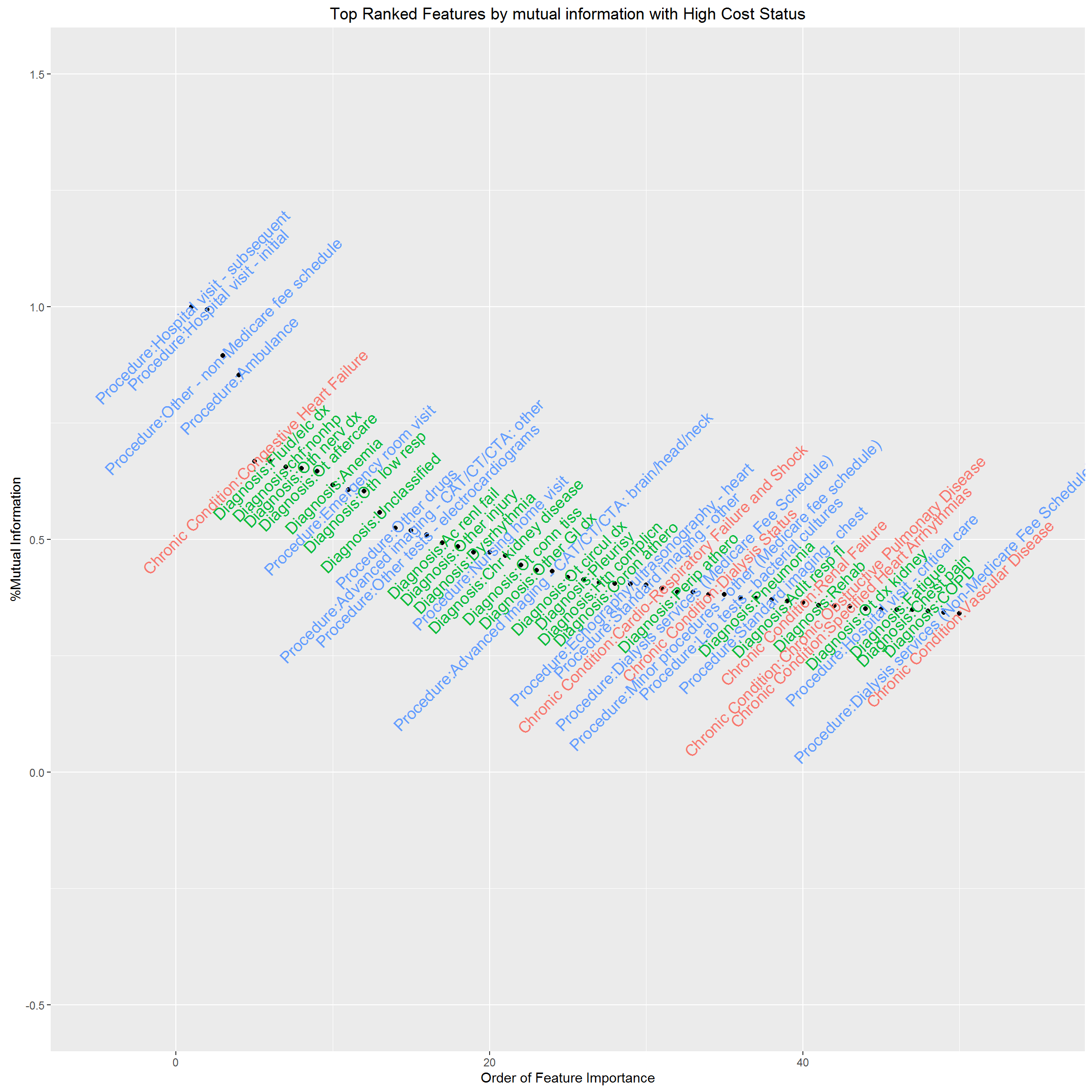
Now, we rank individual clinical feature by “information gain” and visualize feature importance by mutual information. We have standardized mutual information as the ratio to the largest mutual information, therefore, the most important feature in terms of mutual information with high cost status has mutual information %=1. This feature selection helps us decide what features should be included in our predictive model. The results are below.
With these data, we explored a total of five modeling approaches, performing cross-validation to train and test the models. Click on a model below to learn more about our approach.
We compared the performance of the best model given by each approach along measures of accuracy, sensitivity, and specificity. As expected for such high-dimensional data, we found that each of the algorithms had unique strengths in either performance or interpretability.
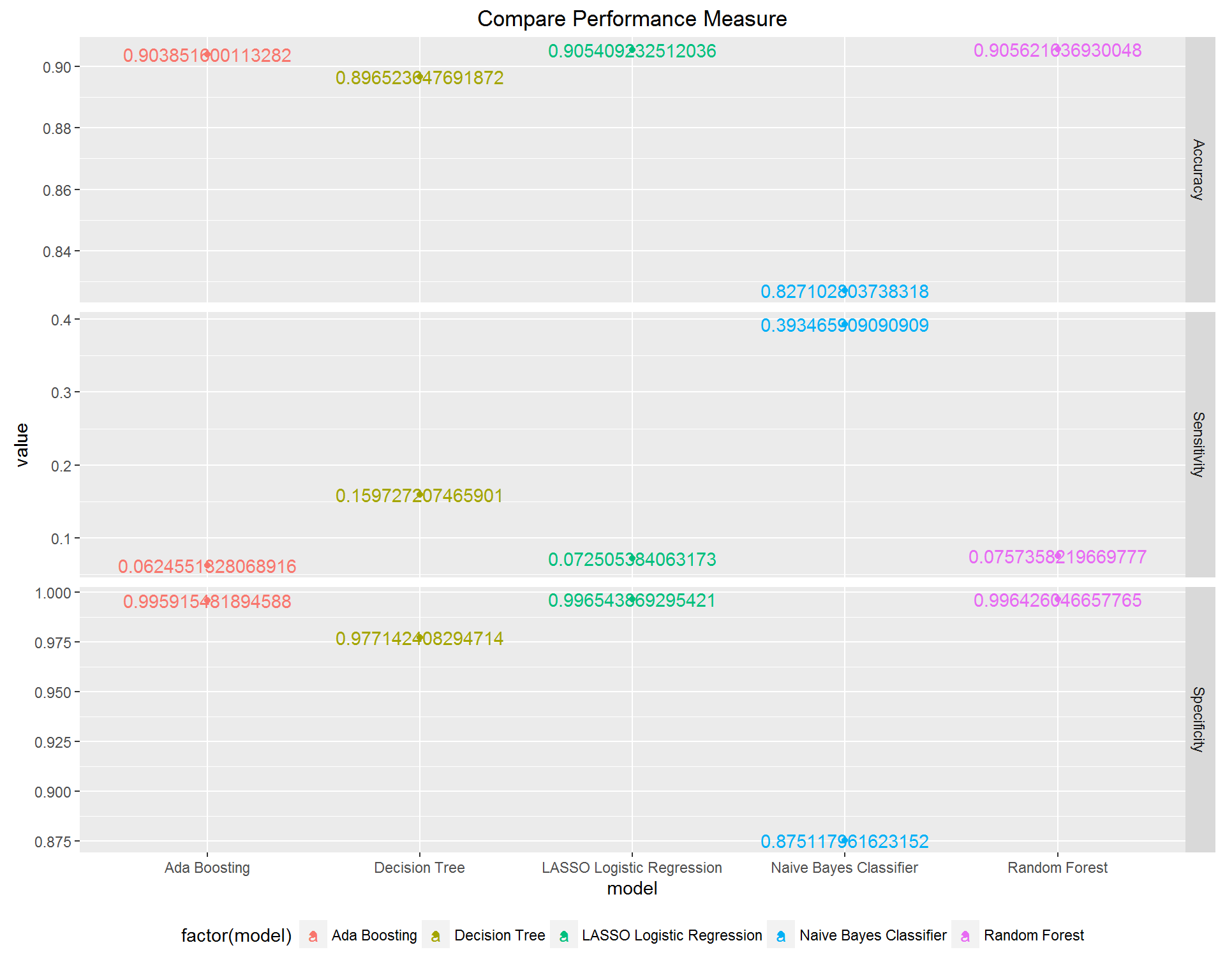
LASSO: it clearly does not yield the best performing model, and in fact, the sensitivity is very low, but an advantage is that the coefficients are interpretable in the same way that the usual logistic regression coefficients are interpreted. E.g., having a certain feature results in an increase in the log odds of being a high cost patient of X amount, where X is the coefficient corresponding to that feature.
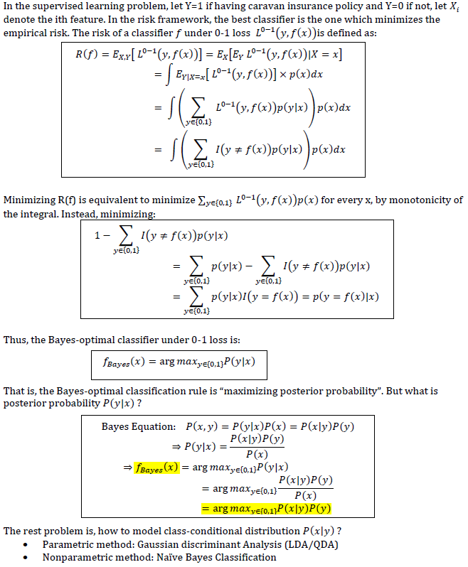
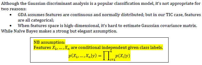
Naive Bayes: based on Bayes’ rule and independence assumption, works surprisingly well, especially high sensitivity rate. However, there is no directly interpretable decision rule that can be drawn from it.
Decision Tree: recursively divides sample space and makes interpretable decision rule, however, the inflexible nature of the division mechanism makes the prediction performance not as optimal as other methods, and in this case, the interpretability is not that good.
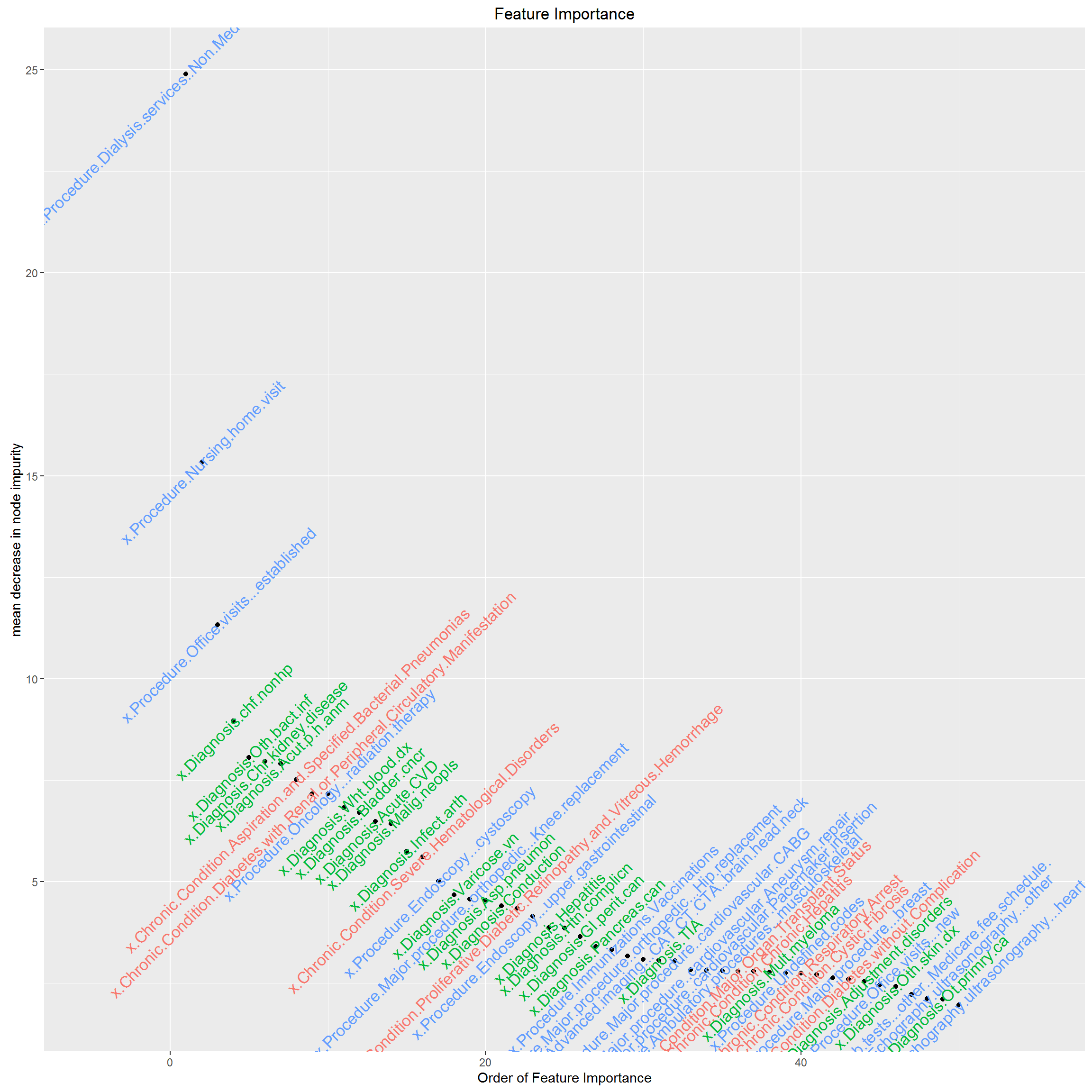
Random Forest: based on two great ideas – Bootstrapping and Ensemble voting, works well which is not surprising. However, the result lacks interpretability.
Boosting: based on the idea of Ensemble voting, has the same disadvantage as RF which is lack of interpretability.
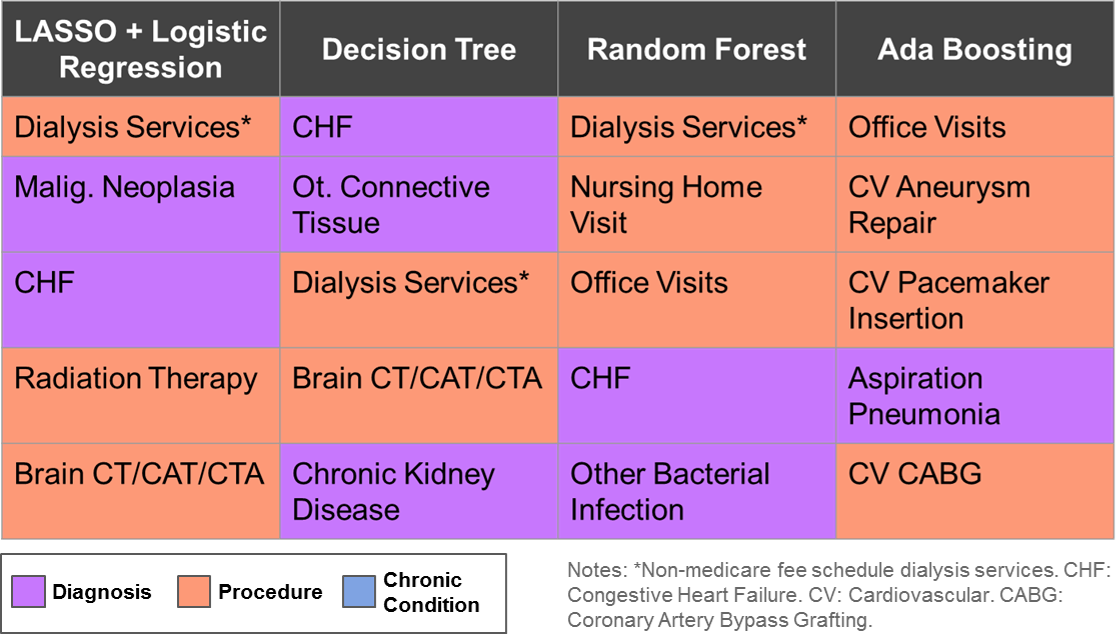
Due to the high dimensionality nature of the problem, no single algorithm excels in all three performance measure and interpretability. But some of them work well enough in the sense that we could have high percentage target rate among true high cost patients cohort, and also overall accuracy. All algorithms have some measure of feature importance, we can compare across them and draw a common set of features, further research is needed to make this project’s result into actionable clinical meaningful evidence.
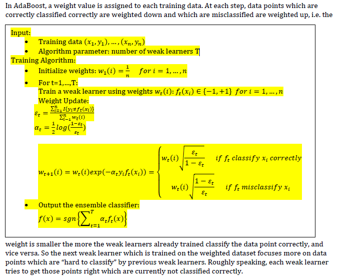 AdaBoost using Desicion Stump as Weak Learner
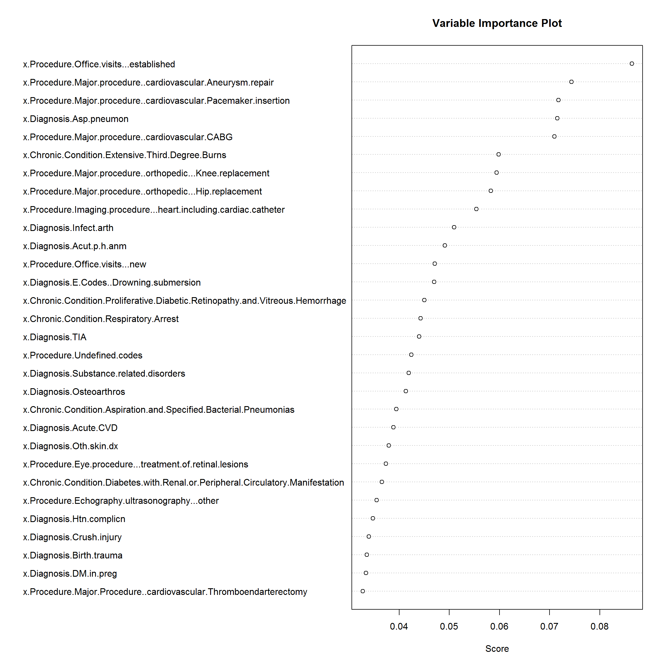
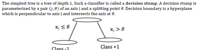 To save computation time,we only include first 100 features selected by entropy. Below is the feature importance.
 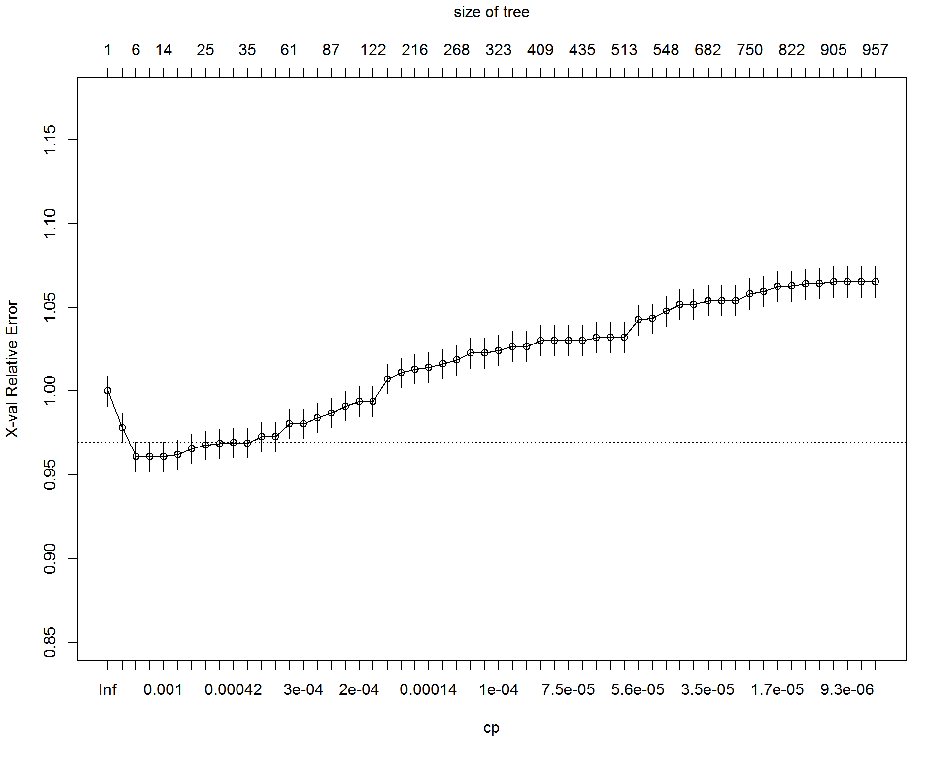 Now we are going to prune the tree using validation set and vizualize the performance.
 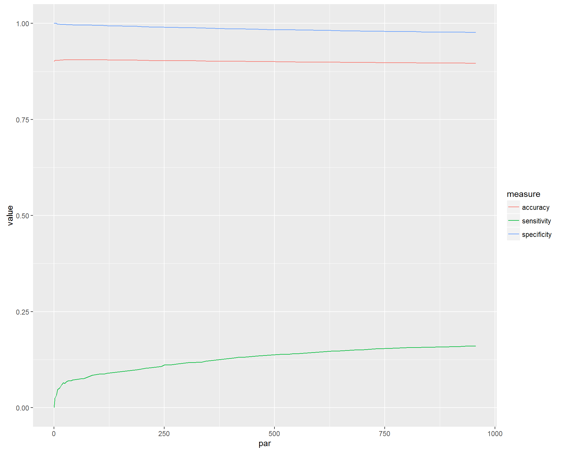 The accuracy is going down with the number of splits increases, this is the problem of over-fitting the training set. But the sensitivity on validation set is going up with the complexity of the tree. Somewhat surprising. We will use the maximum complexity to achieve the maximum sensitivity on independent dataset. Let's prune the tree by sensitivity, predict on validation set, and then visualize performance in terms of entropy.
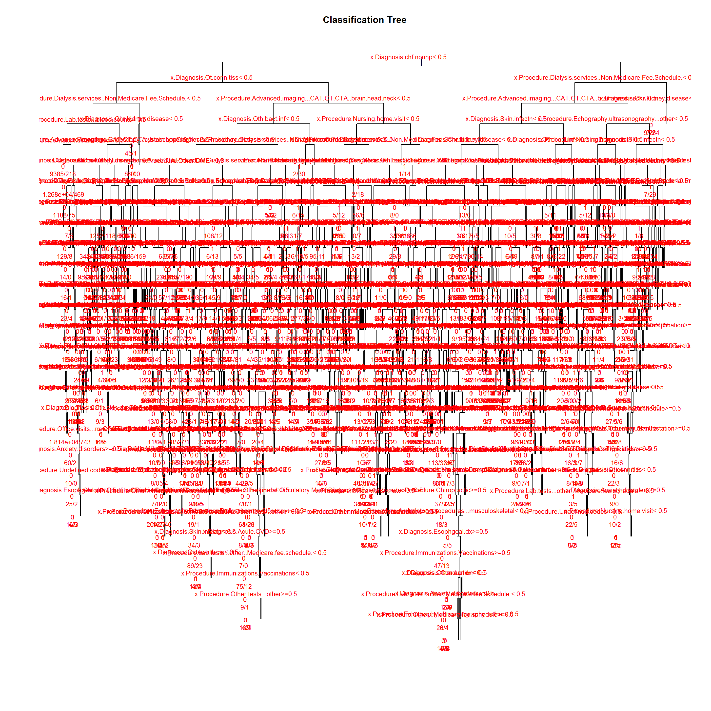
 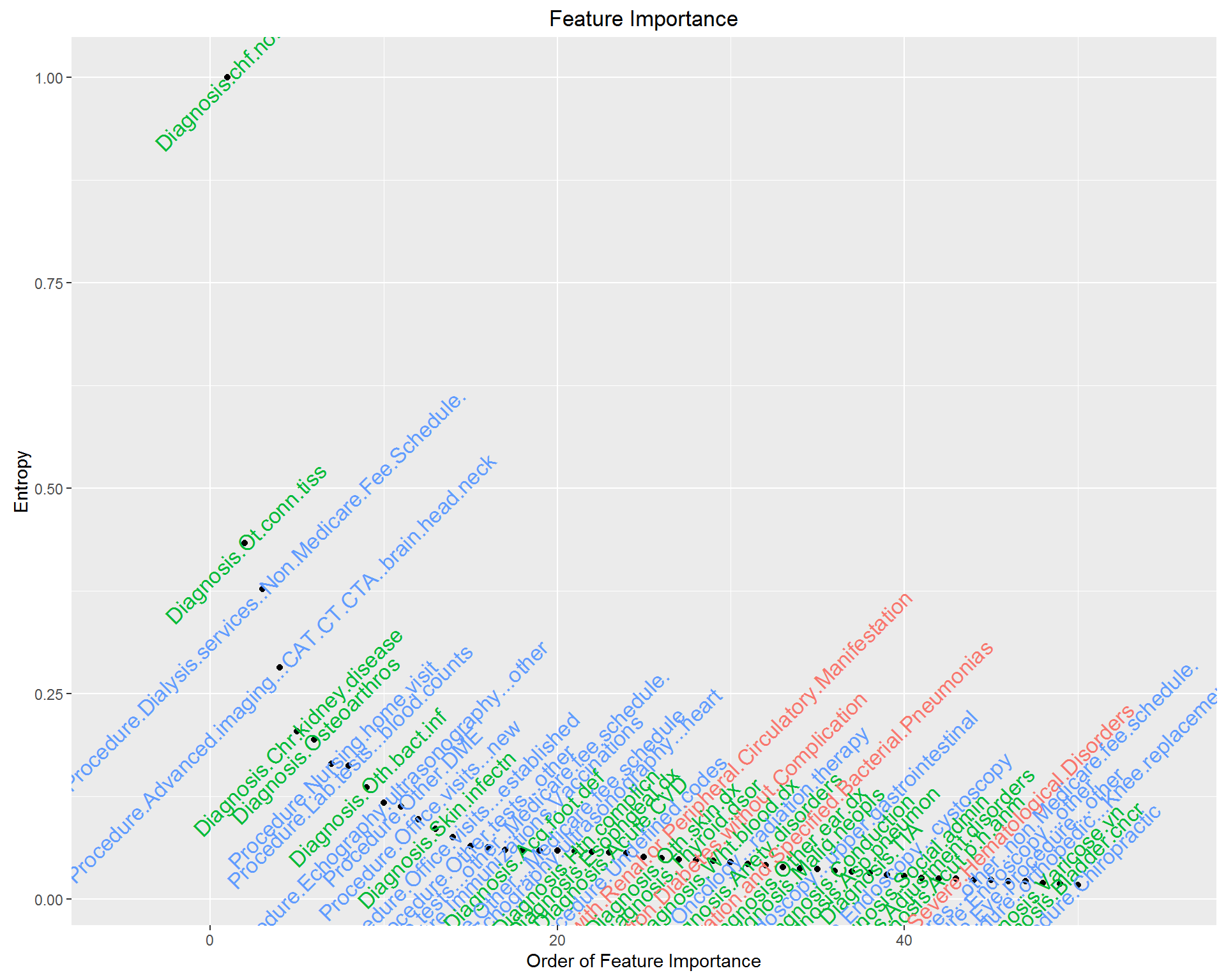 This is our best Decision Tree, which is too complex for interpretation.
 Naive Bayes Model
  We need to model the class-conditional probability distribution for each feature. Since all the features are categorical (binary), the Bernoulli distribution (or multinomial distribution in more general case) is an ideal first choice. We can think of the data sampled following the Bayes model intuitively as two steps. First, Randomly sample a patient from a Bernoulli process with probability p(Y=1), where Y=1 if the patient was high-cost in 2013.Then the patient decide each of his/her feature (among demographic and clinical) from a Bernoulli dsitribution.
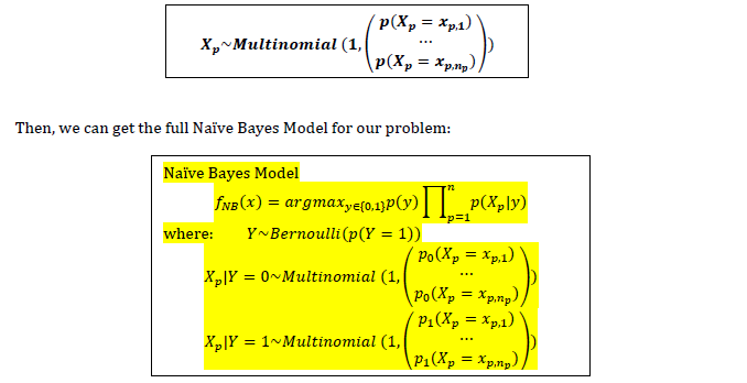 Parameter Estimation
 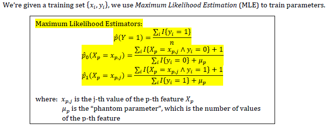 Cross Validation
 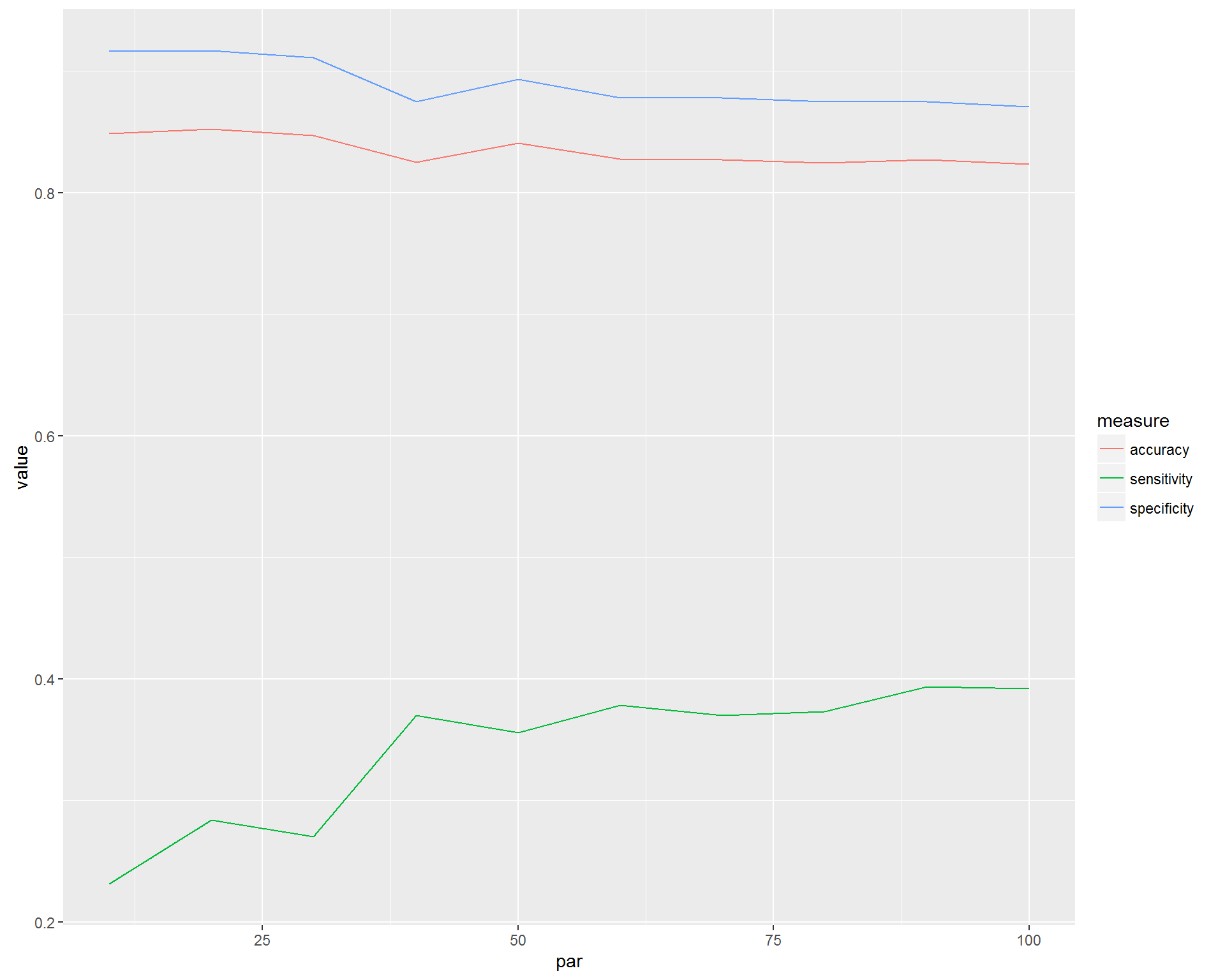 Above is the model performace. For our purpose, what matters the most is sensitivity, that is, how many future high cost patients could be identified correctly. Since if we can identify them, then health care system could provide preventive care to bring potential medical resource utilization down. The accuracy and specificity are all quite stably high in level while number of features included in the model are increasing, therefore, our problem comes down to find the optimal value for sensitivity. Starting from 300+, we could identify 50%+ high cost patients consistently, no matter whether we include 300 or 400 features.
 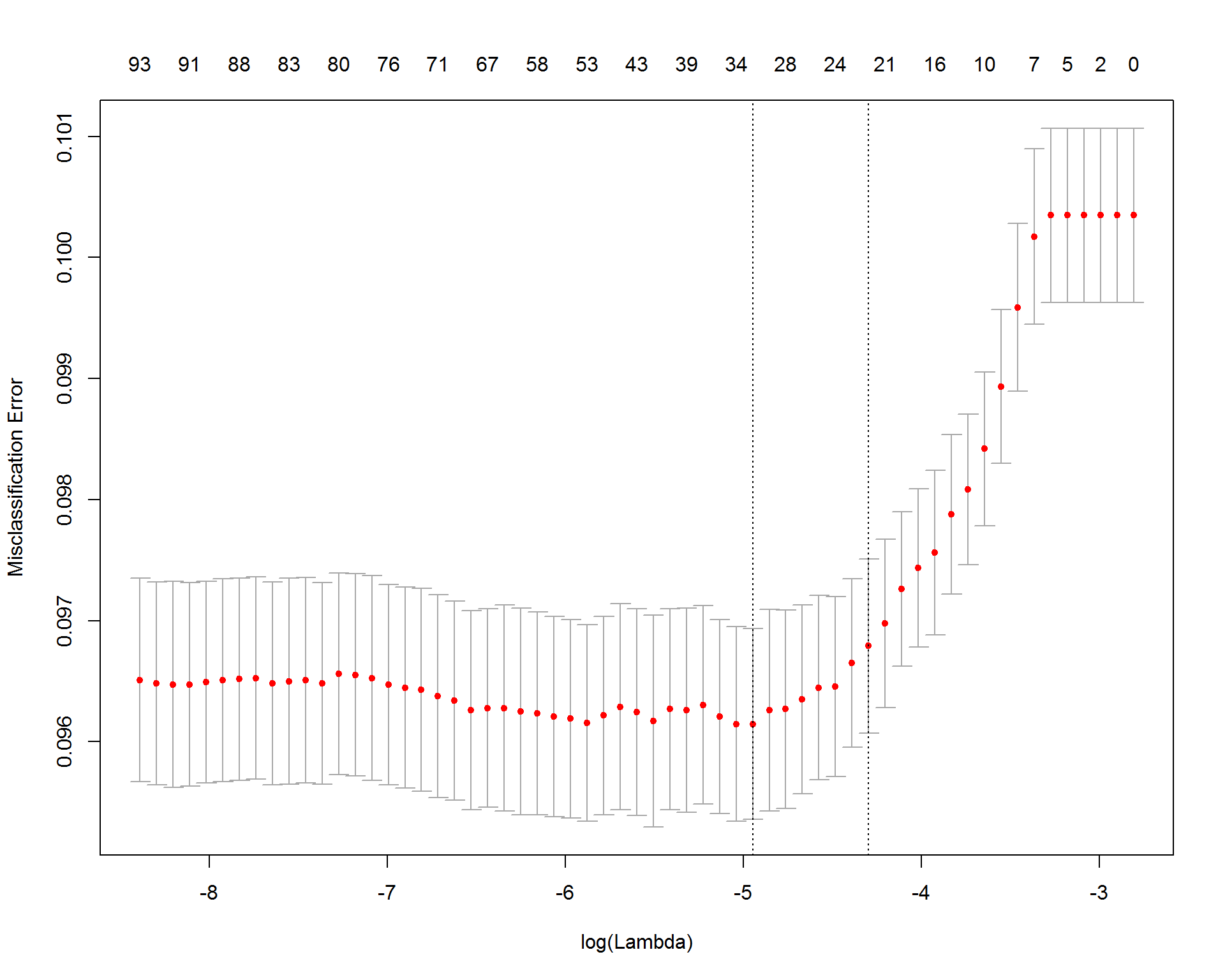 The optimal regularization parameters identified by the cv.glmnet method are shown below. Lmin gives the model with the smallest misclassification error. L gives the most regularized model such that error is within one standard error of the minimum error model. By having a higher degree of regularization, the model given by L is better protected against overfitting, whereas the Lmin has a higher chance of overfitting, but better prediction performance.